2. Molecular Oncology Course - Colorectal Cancer
Analyse Colorectal Cancer using the R2 data analysis platform
This resource is located online at http://r2platform.com/studentcourse
2.1. Introduction
In the late 1980s the Vogelstein model was proposed. It introduced the concept of a stepwise accumulation of genetic mutations leading to the development of colorectal cancer (CRC).

Accumulation of mutations advancing colorectal cancer development
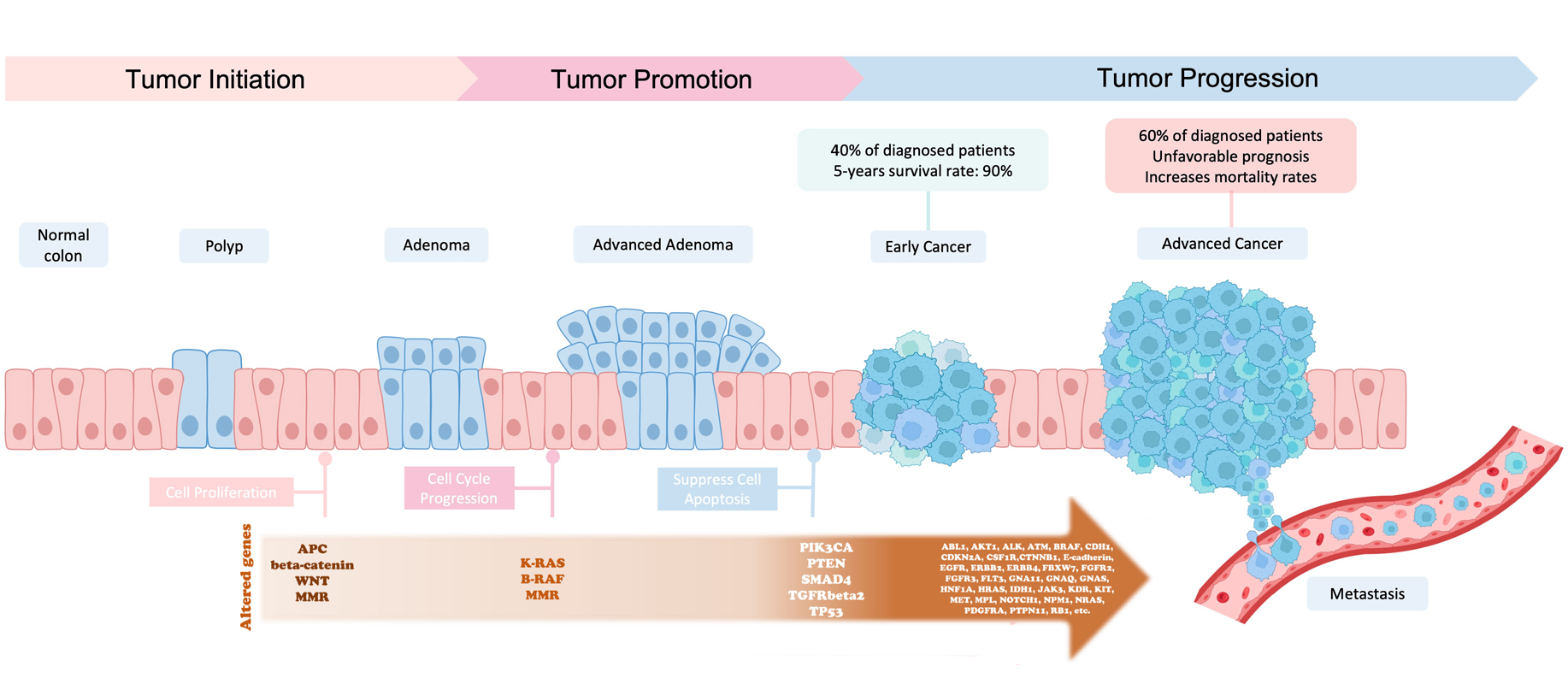
(Figure sources: https://doi.org/10.3390/ijms241311023, https://doi.org/10.1016/j. tranon.2021.101131)
Similar to the picture above, the model highlights the importance of key genetic mutations during CRC progression,
including mutations in APC, KRAS, and TP53. While the Vogelstein model has provided a valuable foundation for
understanding colorectal cancer, subsequent research has revealed that the disease is more complex and heterogeneous
than initially described. Colorectal cancer can involve various genetic and epigenetic changes. Additional
factors, such as the tumor microenvironment, inflammation, and the immune system, also play significant roles in the
progression of the disease.
Colorectal cancer is the third most common cancer worldwide, according to the World Health Organization, accounting
for approximately 10% of all cancer cases, and it is the second leading cause of cancer-related deaths worldwide.
Research is needed to understand the mechanisms underlying treatment resistance and to develop strategies to
overcome it. Better identification and characterization of multiple CRC subtypes could guide treatment decisions and
improve the outcomes for individuals with colorectal cancer. Furthermore, markers for early detection and prevention
might allow for interventions before advanced mutations occur. Clearly it is crucial to understand the diversity and
complexity of colorectal cancer in order to develop new and effective targeted treatment strategies.
Bioinformatics tools enable the analysis of vast amounts of omic and clinical data, helping researchers identify
genetic mutations, epigenetic aberrations, biomarkers, and potential therapeutic targets in order to better understand
and combat cancer.

Web-based genomics analysis and visualization platform R2
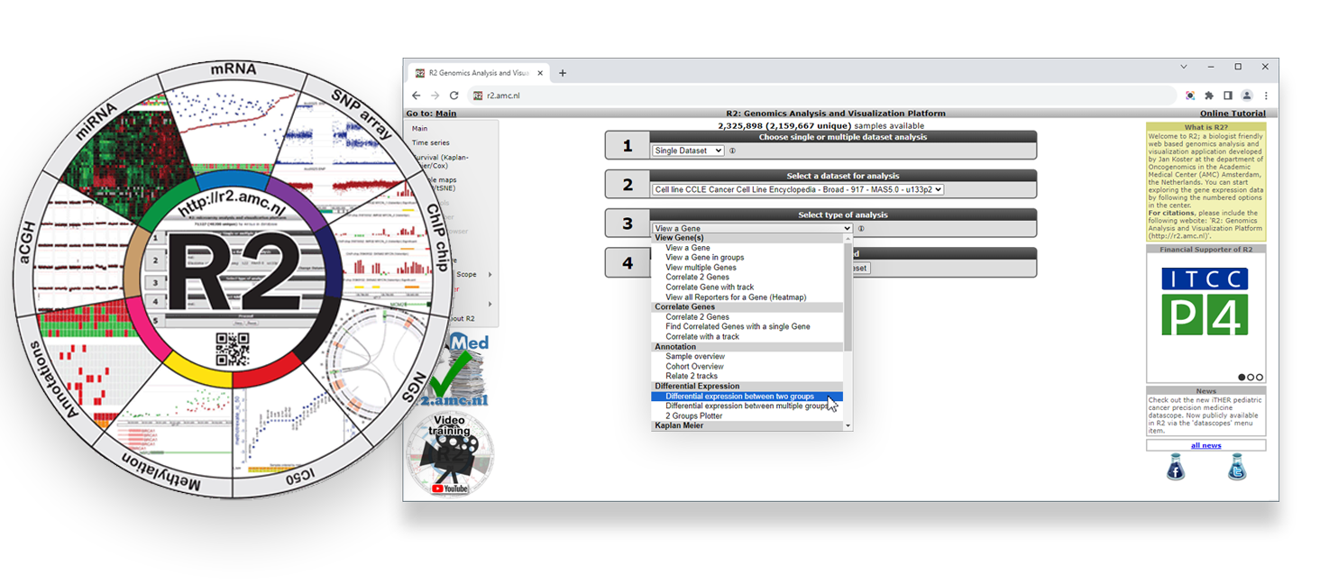
(Figure source: https://r2.amc.nl)
Today you will use advanced bioinformatics tools to explore, analyze and visualize colorectal cancer data in search for a deeper understanding. You will use the freely available and web-based genomics analysis and visualization platform R2, a Core Facility of the Amsterdam UMC. R2 provides the user with many experimental and clinical data sets coupled to a wide variety of clickable bioinformatics tools. Without any coding you will gain hands-on research experience with colorectal cancer omics data and bioinformatics tools.
The in this course will bring you to the R2 platform, often with pre-set settings such that you can pick up an analysis easily. The in this document will open up a Google form, one per section, with which you can submit your answers.
We would like to ask you to fill in the evaluation form about this R2 course during or at the end of the course. To open the form, click the button below:
2.2. Normal colonic epithelium vs adenomatous tissue: a first impression of genomic data
Colorectal cancers are believed to arise predominantly from adenomas. A fundamental query in cancer research consistently revolves around understanding the distinctions between the transcriptomic profiles of normal tissue and tumor tissues. Let’s get acquainted with R2 and its large collection of omic datasets while immediately exploring differences in gene expressions between normal colonic mucosa and colorectal adenomatous tissue.
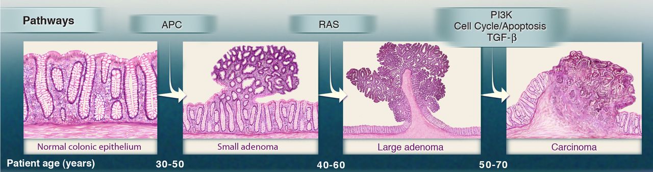
Normal tissue, precancerous adenomas and cancer growth
(Figure source: https://doi.org/10.1126/science.1235122)
Datasets used:
- Mixed Colon - Marra - 64 - MAS5.0 - u133p2
2.2.1. Filtering and exploring
- Open a Chrome browser and find your name behind your assigned number for the student account at the student accounts check in form
- Go to the R2 platform
address: https://hgserver2.amc.nl
Generally speaking, the R2 platform is easily accessible by the link http://r2.amc.nl, but today we work from out developer server hgserver2.
- Sign in with your assigned account that you found in the student account Googledoc.
You’re now on the R2 main page. This genomics analysis and visualization platform contains a wealth of data and
bioinformatics tools to analyze the datasets. Step by step, researchers are guided through a web of options
for data analysis with mostly clickable items. R2’s main page shows this principle: follow the numbered
boxes to develop your analysis of
choice.
We’re first going to see if and how the mRNA expression of several genes changes through the single dataset with the
name “Mixed Colon - Marra - 64 - MAS5.0 - u133p2”.
Datasets have a structured naming in R2, using the following rules: Category + Tissue/ Tumor - author -
number_of_samples_N - normalization - chiptype. In our case the dataset name tells us that the dataset contains
normal and tumor samples (mixed) of colon tissue, that Marra is the author and that there are 64 samples.
- In order to find the dataset in R2, click on the text of the currently selected dataset in box 2.
- A grid pops up that contains all the datasets that are currently available to you. Each row is a dataset and each column contains a different searchable characteristic of datasets. In the bottom right corner of the grid, find the number of rows, i.e. available datasets.
- Under the header Tissue/Tumor type the keyword colon in the white text-field filter, and check the adapted number of rows in the bottom right corner to find out how many colon related sets R2 is hosting.
- Find the RNA expression dataset from Author Marra and click on the row of the dataset that contains 64 samples (N). In the information panel below the grid, you find more information about this dataset. Quickly glance over the summary of the study.
- Select the dataset with a click on the blue box Confirm selection. Check on th emain page in box 2 that the correct set has been selected.
Of course, it is nice to have a lot of RNA expression datasets to analyse and explore, but without proper sample annotation your have very limited analysis options. Let’s explore the annotation for the Marra dataset.
- In box 3, select the analysis type Cohort Overview and click Next.
- In the grid, you can see all the samples in rows, with the available annotation in the columns. Hover your mouse over the pie chart of the tissue annotation and optionally click on a slice to see the Cohort overview adapt to that sample subgroup.
In R2, samples of a dataset can be annotated with e.g. clinical data or biological information. Each group of annotated
data is called a Track in R2. These tracks can be used to filter, color or split data in all types of R2
analyses. The tissue annotation of the Marra set can thus be used to find, for instance, the differences between gene
expression profiles of the adenoma and normal samples.
2.2.2. Find different expression profiles between normal and adenoma tissue
The button below brings you to the form in which you can submit your answers for the first section.
The R2 platform supports a large set of analysis types to explore datasets. One of these modules is the “Find differential expression between groups”. The differential expression analysis aims to identify genes which are significantly different between two groups.
- Click on Main in th eupper left corner.
- Check if you have selected the Marra dataset and in box 3 select type of analysis, Differential expression between two groups_. CLick Next.
- R2 offers a couple of statistical test, in this case we use the T-test which is selected by default.
- Now we have to select which grouping variable to use. Select Group by Tissue (2cat) to use the previously seen tissue annotation. And click Submit.
- An extra field of settings is shown. Select Group 1 normal and Group 2 adenoma. Check that the default Transformation Log2 is selected, and P-value cutoff 0.01. Click Submit.
R2 has generated a large list of differentially expressed genes. On the right hand side of the page you find buttons to follow-up analyses, and underneath the buttons are informative tables about the genes list. One table shows how many genes have higher expression in adenomas compared to healthy tissue and the othter way around.
![]() How many genes were significantly upregulated in adenomas and how many were
downregulated?
How many genes were significantly upregulated in adenomas and how many were
downregulated?
Next to many publicly available datasets, R2 is also hosting a lot of curated lists of genes which we call gene sets. These gene sets can be used to restrict or filter an analysis as well. We can adapt our current search by scrolling down to the end of our gene list. In the Adjustable Settings menu, you can now use a Gene Set to restrict your list.
- Re-generate a list that is specifically associated with colorectal cancer. To do so, hit the Search GS button in the Gene Filters section of the menu.
- Use search field on the top of the table and fill in colorectal, hit enter.
- The KEGG (Kyoto Encyclopedia of Genes and Genomes) database is a comprehensive bioinformatics resource that integrates information about genes, proteins, pathways, and diseases. Click on the triangles in front of KEGG pathways and its subcollections till you find the Colorectal_cancer (62) geneset. Check the set and hit Use selected button.
- Check out the list and see if you recognize multiple genes. You can hover over the magnifying glasses in front of each row to learn more about the genes.
- Now click on the magnifying glass in front of AXIN2 to obtain a scatter plot of the expression of this gene for each sample in the dataset.
- You can see that the plot is split in two. Underneath the plot you can find two annotation tracks, one of which is the tissue track. The colors show the different groups to which each sample belongs. If you hover your mouse over any of the blocks, you can see which side is adenoma and which side is normal tissue. Also note you hoover over the dots in the graph and the tracks to get more information of the individual samples.
- The green bar in the top allows you to easily go to next or previous gene of your list. Click on the arrow with MYC on the right side of the green bar to view its gene expression in the samples.
![]() **What did you observe about the gene expression of AXIN2 and MYC? When you think
about biological processes, why would this be? **
**What did you observe about the gene expression of AXIN2 and MYC? When you think
about biological processes, why would this be? **
The WNT pathway is an important signal transduction cascade which plays an important role in diverse biological processes. The dysregulation of the Wnt pathway has been observed in several cancers including colon cancer.
2.2.3. The WNT pathway
In the next sections we will regularly be using heatmaps to find subgroups of samples or genes that show similar expression profiles. Heatmaps perform unsupervised hierarchical clustering of samples. The algorithm uses the distribution of the (expression) data to find clusters that have similar (expression) profiles and shows the clusters of samples in the plot based on their (dis)similarity. This is combined with the clustering of the genes based on their expression throughout the samples. The heatmap is colored by the z-scores of the samples’ gene expression values. Often annotation tracks are shown above a heatmap. Remember that we can see this annotation but that the heatmap algorithm did not use this information to look for subgroups in the data.
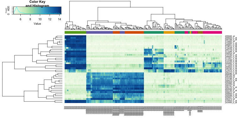
Example heatmap: finding subgroups in your data
- Go back to gene list result page of the previous Differential Expression between two groups analysis, the tab should still be open.
- Generate a list of genes which are differentially expressed comparing normal and adenoma tissue within the KEGG WNT
pathway by adjusting the settings if needed:
- Use the False Discovery Rate for multiple testing correction,
- log 2 values
- and P <0.01.
- First clear the gene set filter with the red cross and use the Search GS button again. Find the KEGG Wnt pathway geneset (hint: use keyword Wnt). Don’t forget to hit Submit in order to redo the analysis with the new settings.
- Use the Heatmap(zscore) button on the right.
![]() Inspect the heatmap did you expect this pronounced clustering?
Inspect the heatmap did you expect this pronounced clustering?
Now let’s generate a Wnt pathway heatmap from a different route:
- Go to the main page
- Select the analysis View Geneset (Heatmap)
- On the next page, select KEGG Gene set Collection. Click Next and then Next again.
- Now scroll all th eway down at the Gene set list and click on Wnt_signaling_pathway. Click Next.
![]() What does the annotation above the heatmap tell you?
What does the annotation above the heatmap tell you?
![]() How and why does this heatmap differ from the previous Wnt pathway heatmap?
How and why does this heatmap differ from the previous Wnt pathway heatmap?
2.3. Identifying groups and their characteristics: CMS
Let us now move past the precancerous stage of adenomas and look at colorectal cancer. Colorectal cancer is a complex and heterogeneous disease, characterized by a multitude of variations in its genetic, molecular, and clinical attributes. This heterogeneity manifests in diverse ways, influencing the tumor’s behavior, response to treatments, and patient outcomes. Understanding this heterogeneity is critical for tailoring effective therapies and improving patient care. In this context, we will explore the various dimensions of heterogeneity in colorectal cancer and its implications for diagnosis, treatment, and research.
In 2015, Guinney et al. (Nat Med. 2015 Nov; 21(11):1350–1356) published a bioinformatics study on a vast collection of colorectal cancer cohorts with detailed molecular annotation. The consortium developed a now widely accepted molecular classification system that allows researchers to categorize most colorectal tumors into one of four distinct and robust subtypes, each characterized by its unique biological features. These subtypes are: CMS1 (MSI Immune), CMS2 (Canonical), CMS3 (Metabolic), and CMS4 (Mesenchymal), see the figure below.
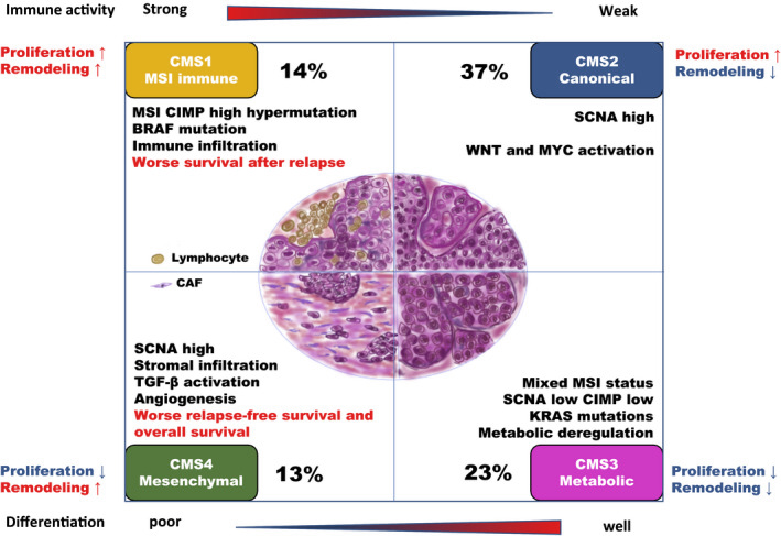
Subtypes in colorectal cancer: CMS classification
(source: http://dx.doi.org/10.1002/ags3.12362)
The button below brings you to the form in which you can submit your answers for the second section.
2.3.1. Clustering with t-SNE maps
An unbiased unsupervised type of clustering analysis is a good starting point to familiarize yourself with a new
dataset. The t-SNE algorithm is an algorithm that was developed in recent years. It finds similarity in expression profiles of
samples and will clump cells with similar expression profiles together on a map. In R2, these mps can be generated
by users with an account. Ones a dataset t-SNE has run, it is available to other users as well. This saves
processing time and costs.
We will use a dataset that was adapted from one of the resources of
The Cancer Genome Atlas (TCGA). They provide a wealth
of omics data: “TCGA generated over 2.5
petabytes of genomic, epigenomic, transcriptomic, and proteomic data. The data, which has already led to improvements in our ability to diagnose, treat, and prevent cancer, will remain publicly available for anyone in the research community to use.”
Dataset used:
- Tumor Colon Adenocarcinoma (students) - tcga - 204 - tpm - gencode36
- In the left side menu on the main page, click on Sample maps (UMAP/tSNE)
- In the grid, filter for the dataset Tumor Colon Adenocarcinoma (students) - tcga - 204 - tpm - gencode36 and click its Select button
Under the graph, a menu allows the user to adapt settings. Colors of the graph points are not set by default.
- Click the button to View standard plot that you can find underneath the little menus
- Find the Color mode dropdown and select Color by Track. Now set the Color track dropdown to use the cms_predicted track, and click Set colors to show the changes.
The most important parameter for the t-SNE algorithm is the perplexity value. The perplexity parameter controls the balance between a focus on preserving local details or global structures of the data. When R2 receives the request to calculate the t-SNE map for a dataset, it immediately calculates and stores the t-SNE maps with different perplexity values. The resulting maps can be found under de setting Versions. It is also possible to show all the available perplexity maps for the dataset at the same time.
- Set Versions to the value all and click Submit again.
![]() What insight did you obtain when you colored the plot with annotation?
What insight did you obtain when you colored the plot with annotation?
![]() Why do you think it is good practice to check different values for a parameter?
Why do you think it is good practice to check different values for a parameter?
Let’s see if there is any difference in survival chances among the subtypes that were shown on the t-SNE map.
2.3.2. Different survival chances for different CMS CRC subtypes?
To see if there is a difference the effect of different survival chancesDataset used
- Tumor Colon (CMS) - Guinney - 3232 - custom - ccrcst1
- In the left side menu on the main page, click on Survival (Kaplan-Meier / Cox)
- In the menu at the center of the page, click at the Dataset setting on the current Dataset name, and find the dataset with Author is Guinney and the amount of samples N is 3232
- Click on the row to read its description in the information box underneath the dataset selection grid
- Leave Separate by at categorical track (Kaplan-Meier) and click Next
- Choose type of Survival *overall and Track lv_cms_final
- Now perform the same analysis, but choose relapse-free instead of overall for the setting type of Survival
![]() What does the first Kaplan Meier plot tell you?
What does the first Kaplan Meier plot tell you?
![]() And what is your conclusion from the second Kaplan Meier graph?
And what is your conclusion from the second Kaplan Meier graph?
2.3.3. Mutations
- From the main page, select the Guinney choose a relate 2 tracks analysis to show the different ratios of mutations per CMS subtype.
- For the y axis choose lv_braf_mut mutations and for the X axis choose lv_cms_final.
- Select the stacked barplot (%) graph type and click Submit
- The Guinney dataset contains several datasets put together. To only look at the samples that looked at the mutational information, scroll down underneath the graph to Adjustable settings menu. Use the Sample Filter with the setting Subset track, select lv_braf_mut and in teh pop up check the boxes of 0 (776) and 1(87), click ok
- For the changes to take effect click Submit
![]() Which CMS group shows the highest amount of Braf mutations?
Which CMS group shows the highest amount of Braf mutations?
Now we will look at the KRAS mutations
- Underneath the graph in Adjustable settings menu, change the y-axis to lv_kras_mut.
- Use the red cross behind the setting Subset track to eliminate the braf mutation subset and click on the dropdown to now select lv_kras_mut. In the pop-up check the boxes of 0 (560) and 1(336), click ok
- Click Submit to see the result
![]() Which CMS group shows the highest amount of KRAS mutations?
Which CMS group shows the highest amount of KRAS mutations?
2.3.4. A dive into CMS1: MSI / MSS in CRC
One of the characteristics of CMS I is MSI instability. Genomic instability in colon cancer can be divided into at least two major types: microsatellite instability (MSI) or chromosomal instability (CIN). Microsatellite instability (MSI) is caused by mutations in DNA mismatch repair genes such as MLH1, MSH2, MSH6, and PMS2, and it is found in 10% to 15% of sporadic colorectal cancers (CRCs). The presence of MSI predicts a good outcome in colorectal cancer.
In MSI colon cancer, genes of the DNA mismatch repair system play an important role. Germline mutations in these genes are a major cause of the inherited form of colon cancer, namely HNPCC (hereditary nonpolyposis colon cancer). In sporadic forms of colon cancer however, these genes are frequently inactivated. Inactivation is often achieved via hypermethylation, switching the gene off. Hypermethylation of genes in colon cancer is most common in colon tumors with a proximal location in the colon and much less in colon tumors with a distal location.
Dataset used: The next section we will use another dataset. * “Colon Tumor - Watanabe - 84 - MAS5.0 - u133p2”*
This dataset consists of Microsatellite stable (MSS) tumors and microsatellite instable (MSI) tumors.
MSS vs MSI
- Find the dataset Tumor Colon - Watanabe - 84 - MAS5.0 - u133p2 and read the Summary in the information panel underneath the dataset selection grid. Then Select the dataset.
- Use the Differential expressed genes between two groups module to generate a list of differentially expressed genes between MSI and MSS characterized tumors (MS_status). Because we know that DNA repair genes play an important role in microsatellite (in) stability, we can use a set of DNA repair genes to examine whether these genes indeed are differentially expressed between MSI and MSS tumors and which genes exactly make the difference. With the Search GS button, filter for DNA repair genes, and find them in Categories. There are 247 genes annotated as DNA repair genes. Perform the analysis.
![]() Which gene is on top of the list?
Which gene is on top of the list?
- One of the genes that is differentially expressed, is MLH1. Click on its magnifying glass to look at the expression of MLH1 in the MSI vs. MSS samples.
![]() In the list of differentially expressed genes, MLH1 is significantly lower
expressed in the msi group vs the mss group: msi < mss. When you look at the expression plot of MLH1, what do you
notice about the expression of the samples in this group? Do you see a clear-cut trend of lower MLH1 expression in the
MSI group?
In the list of differentially expressed genes, MLH1 is significantly lower
expressed in the msi group vs the mss group: msi < mss. When you look at the expression plot of MLH1, what do you
notice about the expression of the samples in this group? Do you see a clear-cut trend of lower MLH1 expression in the
MSI group?
MSI tumors give a very heterogeneous picture. This could be an indication that within the MSI tumor group also a subgroup could be identified.
- Hover with your mouse over data points or inspect the annotation underneath the graph to see if you can identify a subgroup of an annotation track in which low MLH1 expression occurs more often.
- Scroll down to the Adjustable setting and change grouping setting _Track into **MS_orientation. To visuallly support the distinct group, also change Color mode to Color by a Track and choose the same track to color the plot. Click Submit
R2 has an analysis tool called relate two tracks where you visualize the relation between dataset annotations.
- Go back to the main menu and select relate two tracks and click Next.
- Select for the X-track the MS_status and for the Y_track Orientation and click Submit.
- In the MLH1 expression graph we saw that low gene expression was not equally distributed within the MSI group. Let’s add this layer of information in this plot as well: select Color mode Color by a Gene and enter MLH1 as gene to color the plot. Click Submit.
![]() Concluding, with which two characteristics can you describe the subgroup that
more often has a low MLH1 expression?
Concluding, with which two characteristics can you describe the subgroup that
more often has a low MLH1 expression?
In many cases of proximal colon cancer with MSI, the high level of microsatellite instability is caused by the loss of MLH1 expression. MLH1 inactivation can occur due to mutations in the MLH1 gene or through epigenetic changes, such as promoter methylation. In summary, the loss of MLH1 expression is a common mechanism leading to MSI in proximal colon cancer. Understanding the relationship between MLH1 expression and MSI is crucial for diagnosing MMR (mutation mismatch repair) deficiency, predicting prognosis, and guiding targeted therapies for patients with colorectal cancer.
So we have identified an important player as discussed in college. We identified this key player in the Watanabe data set. We will now corroborate our findings in another dataset. Not only because this is an old set (look upthe background information in the information panel of the dataset selection grid), but it is common practice in to validate your results with other sources. We will use a dataset that we already looked at with the t-SNE clustering algorithm.
MSI in tcga set
- Select Tumor Colon Adenocarcinoma (students) - tcga - 204 - tpm - gencode36
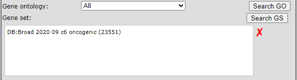
- Perform the Differential Expression between two groups analysis for Microsatellite_instability (no vs yes), and select with the Search GS button the Broad 2020 09 c6 oncogenic. Submit
- Click again on the MHL1 gene magnifying glass.
Don’t forget to use the filter option
So in this set too MLH1 seems to play a key role and is possibly affecting other genes.
One way to find out which genes are possibly regulated by the MLH1 gene is to find genes which are (inverse) correlated with this gene.
Find genes correlating with a single gene
- From the main page, run the Find Correlated Genes with a single Gene module for the MLH1 gene. Use again the filter option for the Broad 2020 09 c6 oncogenic geneset.
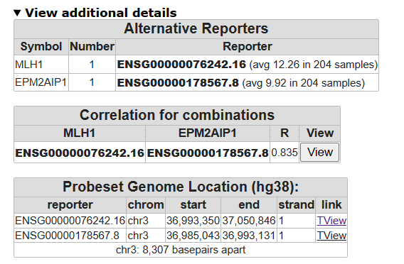
- Then click on the best correlating gene to plot both genes together, in a two gene view. Inspect the correlation. Can you think of reasons why the gene expression is highly correlated/
- Click on view additional details, on which chromosomes are both genes located
- Click T-view and zoom out 2 times
The Genome Browser allows you to “walk over the genome”. Underneath the genome locations are annotated with the genes that are located at the specific location. Genes colored in red are read in reverse direction.
![]() What can you say about their location of the two genes?
What can you say about their location of the two genes?
The correlating genes result page shows two columns: the positively correlating genes on the left, the negatively correlated genes on the right. Let’s have a closer look at this last group.
- Go back to your genelist of correlating genes and scroll down to the Adjustable Settings menu at the bottom of the page. Adapt here the setting Corr. r cutoff sign to only look at the negatively correlated genes. Hit the red cross of the Gene Filter and click Submit to update the result page. This might take a while.
- Click the button on the right side of the page Chromosome map.

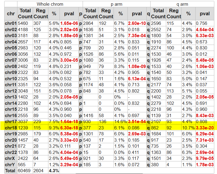
The overrepresentation is calculated of genes that negatively correlate with MLH1 expression with respect to all genes present on (an arm of) a chromosome.
- A lot of genes are clearly over-represented on a number of chromosomes, especially chrom 18 with a high p-value.
![]() Which chromosomes show extreme significance in gene overrepresentation?
Which chromosomes show extreme significance in gene overrepresentation?
Now let’s see How strong MLH1 expression is associated with CMS subtypes.
- From the main page select the Correlate a Gene with a track analysis to confirm the strong association of MLH1 expression with the CMS1 subtype.
DNA methylation
The R2 platform hosts a variety of dataset types. Not only gene expression datasets but also methylation arrays can be found.
- Go to the main menu and select the dataset Tumor Colon adenocarcinoma - tcga - 296 - custom - ilmnhm450
- Create the View a gene plot for MLH1
- Under the triangle of View additional details click on the view all link.
- Scroll down to the bottom of the page to make a Subset track selection with microsatellite_instability to only select the samples that have been annotated for this characteristic (yes and no). Click Next.
A heatmap is generated of methylation levels. Each column corresponds to a sample, and each row corresponds to a feature (a single CpG site or a larger target region including multiple CpG sites, e.g. promoter regions). A hierarchical clustering of the samples is performed. The MLH1 reporters themselves seem faulty, but in you find CpG sites above that are located at the promotor sites of MLH1 and the gene that we have seen before as strongly correlating in expression.
- Hover with your mouse over the r2_at_cms track to see to which cms subtype the cluster of hypermethylated samples belong.
![]() Which cms group did you find?
Which cms group did you find?
![]() Why are we looking at methylation levels around the promotor of MLH1?
Why are we looking at methylation levels around the promotor of MLH1?
2.3.5. What pathways drive subtype CMS4?
Previously we looked into CMS subtype 1. Let’s now have a look at the other subtypes. We would like to understand what sets CMS 4 apart from the subtypes 2 and 3.
- On the main page, select Tumor Colon Adenocarcinoma (students) - tcga - 204 - tpm - gencode36
- Choose the analysis Differential Expression Between Two Groups.
- Choose the track cms_predicted and look at groups **cms2 and cms4
- The analysis can take a while.
Gene set analysis helps researchers interpret the biological relevance of a group of genes. Instead of looking at individual genes, it allows you to understand the collective functions or pathway involvements genes in your list. This can provide more meaningful insights into the underlying biology of a particular condition or experiment.
- Click on the top most button on the right that is labeled Gene set analysis.
- Select the Gene set Collection Broad 2020 09 h hallmark
- Switch the Representation setting to all to look at both over- and under-representation
- Click Next
![]() Which gene sets do you see pop up and are they over or under expressed in CMS 4?
Which gene sets do you see pop up and are they over or under expressed in CMS 4?
![]() Explain the biological relevance for the CMS4 subtype for these over- or/and underexpression of these gene sets for CMS4 subtype CRC tumors
Explain the biological relevance for the CMS4 subtype for these over- or/and underexpression of these gene sets for CMS4 subtype CRC tumors
2.4. Effects of imatinib: shifts of signature profiles and molecular subtypes
Mesenchymal Consensus Molecular Subtype 4 (CMS4) colon cancer is associated with poor prognosis and therapy resistance. In this proof-of-concept study, Kranenburg et al. assessed whether imatinib could shift cms4 subtype specific characteritics.
The button below brings you to the form in which you can submit your answers for the third section.
We want to see how the expression changes between the pre- and post-treatment samples’ expression of specific mesenchymal genes such as ZEB1, PDGFRA, PDGFRB, and CD36 :
- On the main page in the center menu, select the dataset Tumor ImPACCT - Kranenburg - 30 - custom - ensh37e75
- Choose the analysis View Multiple Genes and click Next
- In the Genes/Reporters to include textbox, type Zeb1,PDGFRA,PDGFRB,CD36
- Set Track to pre-post-imatinib to divide the samples in the pretreatment and the posttreatment group and Handle groups by lump by gene plot group to show this per gene.
- Set color by to Track in order to make the box plots visually more distinct.
- Click next
![]() What can you say about the level of expression of these genes post treatment?
What can you say about the level of expression of these genes post treatment?
![]() As with every result, think about why you see the result - does it make sense,
what is the biological implication. So, in this case, what is the role of ZEB1 in EMT? (Use Google or another informative source)
As with every result, think about why you see the result - does it make sense,
what is the biological implication. So, in this case, what is the role of ZEB1 in EMT? (Use Google or another informative source)
2.4.1. Proliferation vs metastases
Mesenchymal tumor phenotypes are generally accompanied by reduced proliferation. Indeed, high expression of proliferation signatures and Wnt target genes are associated with good prognosis and reduced metastatic capacity in CRC
- On the main page, make sure that the selected dataset is Tumor ImPACCT - Kranenburg - 30 - custom - ensh37e75
- Select the analysis View Geneset (Heatmap)
- Select Gene set Collection Broad 2020 09 h hallmark and click Next
- Click Next again
- Click one time on Gene set HALLMARK_MYC_TARGETS_V1 (200) and click Next
The heatmap for the z-scores of the expression values of the MYC targets geneset is shown. Underneath the heatmap you find the geneset average z-value per sample, also known as the signature score. With an account you can save such scores as a Track to use further analyses in R2.
- Click on the store link in the small table, a bit underneath the heatmap.
- In the page that pop-ups, you can adjust settings
- Check the name that is provided for this signature score: _hallmark_myc_targets_v1 and read the description
- We leave everything as is and click on Build set
- Go back to the main page
- Click Relate 2 tracks, click Next
- Select x-axis pre-post-imatinib and y-axis hallmark_myc_targets_v1_signsc
- Select Graph type Box/dot plot (bands)
- Change Color mode to Color by Track and click Submit
- Do the same route (starting with View Geneset(heatmap)) for the Wnt target gene set WNT_ImPACCT (student) that you can find in the gene set collection My R2 Communities and store the signature score as a track as well.
- Go back to the Relate 2 tracks just as in the previous exercise.
- In the Adjustable settings menu underneath the plot, change the y track to wnt_impacct
- Again relate this signature score with the track pre-post-imatinib
- Optionally change the Graph type to another type that you want to try out
- Click Submit
![]() What happened with the expression of WNT- and MYC-target genes post treatment?
What happened with the expression of WNT- and MYC-target genes post treatment?
![]() Even though it is counterintuitive, can you think of a reason why this actually
could be a better outcome than before treatment?
Even though it is counterintuitive, can you think of a reason why this actually
could be a better outcome than before treatment?
2.4.2. Assess the prognostic value of imatinib treatment
To assess the potential prognostic value of the treatment, we will make a signature of the genes that were changed after treatment.
- On the main page, make sure that the selected dataset is Tumor ImPACCT - Kranenburg - 30 - custom - ensh37e75
- Select the analysis Differential expression between two groups
- Switch the Group by setting to pre-post-imatinib and click Submit
- Extra settings appear. We can now fill in the groups for which we want to find the differentially expressed genes: Group 1 pre-imatinib (15) and Group 2 post-imatinib (15)
- Set the P-value cutoff to a stricter value: 0.001 and click Submit
A table shows the differentially expressed genes. On the right underneath buttons with followup analyses, you can find a small table that shows how many genes were downregulated by the imatinib treatment (imatinib: pre-imatinib >= post-imatinib) and how many genes were upregulated (imatinib: pre-imatinib < post-imatinib).
![]() How many upregulated genes were found?
How many upregulated genes were found?
- To use this genelist in other analyses within R2, click on the lowest button on the right side that is labeled Store result as custom gene set
- As a name, type impacct_imatinib_treatment_up
- In the Included groups check only the upregulated genes
- Click on Save gene set
The treatment resulted in a shift in gene expressions. To find out what the effect is of this shift, we will make use of the geneset of upregulated genes that we just saved, now in combination with the Guinney dataset, the cohort dataset with annotated CMS status and survival data. We use the unsupervised k-means algoritm to find groups in our cohort that show similar expression patterns for our geneset.
- On the main page, select the Guinney dataset again
- Select the K-means analysis in box 3 and click Next
- In the Subset track dropdown, select lv_stage, and in the pop-up window check the boxes 2 and 3 , click Ok
- Behind the setting Gene set, you find the button Search GS. Click on the button and find your previously stored gene set under User gene sets > - > impacct_imatinib_treatment_up and hit the green button on the left to use the selected gene set
- We leave the number of groups at 2
- Set the Cell width to 1 and Cell height to 8 and click on Next
The Kmeans algorithm looks at the expression of the samples for the selected genes and makes two groups of samples that show most similar expression patterns. Then for each gene it shows the expression by a color code
![]() Which color group would you say shows high expression and which color group shows
low expression of the geneset? (Thus, high: yellow or purple and low: yellow or purple)
Which color group would you say shows high expression and which color group shows
low expression of the geneset? (Thus, high: yellow or purple and low: yellow or purple)
Again this group division can be stored in R2 to use in a next analysis.
- To do so, hit the button Store as track that you can find on the left
- On the following page, just click the button Next
- To save the results in a way in which we will easily remember what the track was for and which group showed which expression, change the name of Group ‘cluster 1’ into high and of Group ‘cluster 2’ into low. Also change Track name into kmeans_imatinib_induced
- Click on Build set and go back to the main page
Let’s see which cms subtypes are represented in the two k-means sample clusters
- On the main page, select the analysis Relate 2 tracks
- For the X track scroll all the way down and select kmeans_imatinib_induced
- For the Y track choose lv_cms_final
- In the Subset track dropdown, select lv_stage, and in the pop-up window check the boxes 2 and 3 , click Ok
- Change the Graph type into Stacked bar plot (%)
- Order Groups by group size and hit Submit
![]() If the impact of imatinib shows a shift of the geneset from low expression to
high expression values, what shift in CMS subtypes do we expect to see?
If the impact of imatinib shows a shift of the geneset from low expression to
high expression values, what shift in CMS subtypes do we expect to see?
![]() What is known about the treatability of subtype 4 and cms 2 respectively?
What is known about the treatability of subtype 4 and cms 2 respectively?
- From the main page in the left menu click the Survival (Kaplan Meier/Cox) analysis
- Check that the Guinney set is selected and that the separation is made by a categorical track. Click Next
- Choose overall survival type and Track kmeans_stage23_imatinib_induced. Click Next
- In the left menu click again the Survival (Kaplan Meier/Cox) analysis
- Repeat the process but select the relapse free instead of overall survival type.
![]() What is your conclusion?
What is your conclusion?
2.5. Identifying key drivers of CRC: superenhancers controlling gene expression
An enhancer is a 50-1500 bp region of DNA where activator proteins, such as transcription factors, bind and that
increase the likelihood transcription will occur at a gene. They can be located up to 1 Mbp away from the gene,
either upstream or downstream from the start site, and either in the forward or backward direction. A super-enhancer
consists of multiple enhancer regions. This larger region is bound by more transcription factor proteins to drive
transcription of genes. They can be up to 20 times the size of an enhancer.
In chapter Integrative analysis: ChIP-seq data of the R2 Tutorial, you can find a more detailed description of Chipseq data analysis.

The histone modifications of active promoter sites and (super-)enhancers of a gene
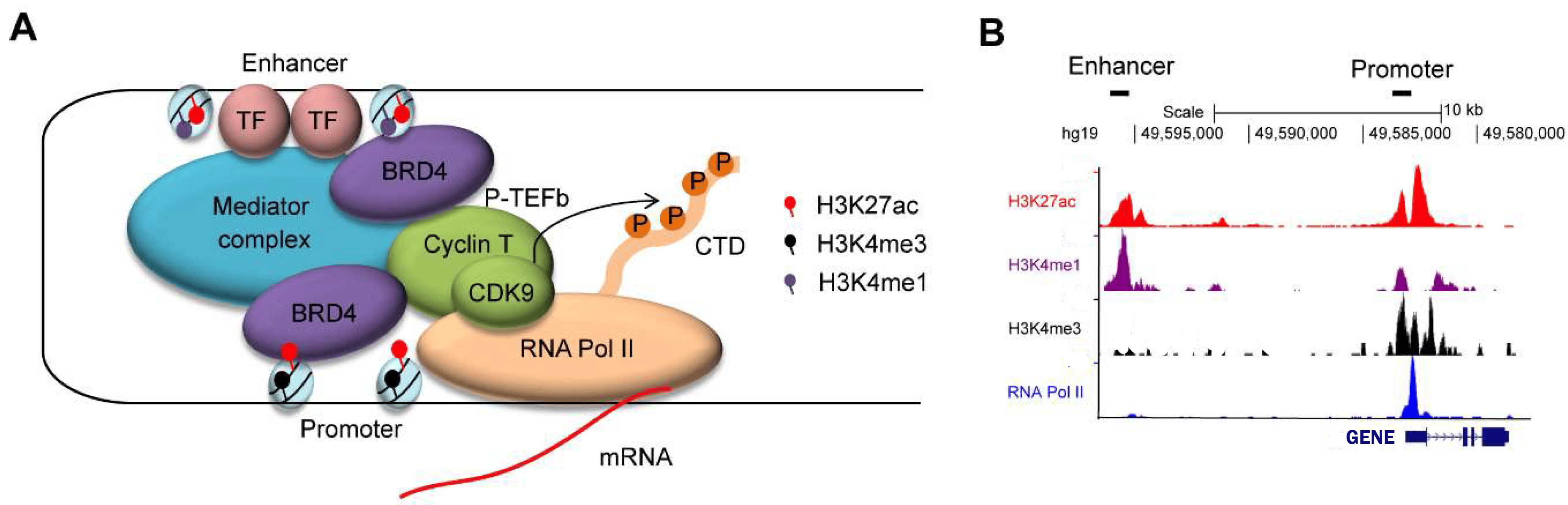
Enhanced enhancer activity can lead to the overexpression of oncogenes, which promotes cancer growth. Super-enhancers often play a central role in determining cell identity and tumor initiation and progression. Identifying these active enhancers can help pinpoint key drivers of colorectal cancer, potentially revealing new therapeutic targets.Different patients may have colorectal tumors with distinct enhancer landscapes. By characterizing enhancer activity, researchers can potentially classify patients into subgroups with different treatment responses or prognosis, enabling personalized medicine approaches.
With Chromatine Immuno Precipitation binding of elements to the genome can be studied. Transcription of DNA to RNA
is regulated by the binding of these elements. These can be Transcription Factors, that bind temporarily to start
transcription, but also chemical modification of the histones (molecular structures that coil the DNA) by methylation, acetylation, etc. These modifications change the accessibility of the DNA for transcription.
When a specific antibody is used in ChIP-seq that recognizes these chemically modified regions, these specific
regions can be studied. Regions with H3K27Ac acetylation mark active enhancers and active promotors (i.e. active
transcription), H3K4Me3 methylation marks active promotors. Studying the relative contributions of both types of
modifications allows a researcher to discern enhancer regions from active transcription sites.
- From the main page select the analysis ChIP Genome Browser and click Next
You are now at the GenomeBrowser at the genomic location of mycn.
Regions encoding genes are drawn at the bottom of the graph. When in red they’re encoded in the reverse direction,
coding exons are darker.
Li et al. (2021) sequence 73 pairs of colorectal cancer tissues and generated 147 H3K27ac ChIP-Seq, 144 RNA-Seq, 147 whole genome sequencing and 86 H3K4me3 ChIP-Seq samples. The patients were classified into the 4 CMS subtypes. Therefore, we now have gene expression and chipseq data of this CMS classified patient cohort. Because it is difficult to look at many profiles at the same time, we averaged the data per cms group. This way we created so called ChIP seq meta profiles. Let’s load them into your Genome Browser
- In the right upper corner, click the button Load / Store Profile
- In the Profile dropdown, seelect student - Li_CRC_normal_tumor_cms1234 and click Execute.
- Click On the top button Goto the GenomeBrowser
You now see the meta profiles of normal colon tissue, and CMS 1 to 4 meta profiles. For each group you see both H3K27ac and H3K4me3. If you scroll down, you can see that you are at the location of the MYC gene. At an active promotor site, you will find H3K4me3 peaks. You will also find peaks in the H3K27ac profiles at that location. But at an active enhancer site, you will only find H3K27ac, no H3K4me3. Thus left from the myc gene location, you see H3K27ac peaks without H3K4me3, and that is a known superenhancer location of MYC. Let’s look for more superenhancers:
- In the left upper corner, you can write the name of a gene and you will be taken to its location on the genome. Type ascl2 in the textfield and click Go
- Click the View button (if there are more View buttons, just take the top one) and scroll downn to check that you have arrived at ASCL2.
- Now we need to zoom out to find possible superenhancers. Zoom out 10x with the button on top of the page. Then zoom out 5x. Do you see an area with high peaks of H3K27ac where no H3K4me3 can be found? There is a superenhancer.
The difficulty is that you never know how far away from the gene the superenhancer is located. Also, it can be upstream or downstream from the transcription start site of the gene. And… you might even find enhancer regions in the introns of some oncogenes.
Lastly, above the ChIP-seq profiles, you can also find the averaged z-score of the gene expression of the subgroups
of patients. Hover your mouse over the colored dots to see to which group they belong and of which gene it shows the
average expression. This way you can see whether the expression itself differs between the CMS groups, and between
normal colon tissue and tumor tissue.
Ideally you should find oncogenes or transcription factors that are differently expressed in tumor tissue and normal
tissue, and also show different enhancer profiles between normal and tumor tissue.
![]() Play around with the GenomeBrowser. Look for genes that you might remember from
the lectures and see if you can find superenhancer areas. Also check if you can see differences between the CMS
groups, and try to explain the differences. Did you find an interesting gene and how much did you need to zoom out?
Play around with the GenomeBrowser. Look for genes that you might remember from
the lectures and see if you can find superenhancer areas. Also check if you can see differences between the CMS
groups, and try to explain the differences. Did you find an interesting gene and how much did you need to zoom out?
- If you need some inspiration, you could check out genes from this list: IL20RA, LIF, IER3, PLAGL2, FAM3D, TNS1…
- Search the internet as to why these could be interesting genes to look up.
2.6. Optional exercise: Experiments TP53 - Molecule of the year 1994
Nearly half of human malignancies harbor mutations in tumor suppressor gene p53, mutations that facilitate and promote metastasis, tumorigenesis, and resistance to apoptosis.
These mutations generally lead to loss of DNA binding and an inability to transactivate canonical anti-proliferative p53 target genes. Genotoxic chemotherapeutics, like doxorubicin and etoposide, are clinically relevant activators of wild-type p53, but the potential risk of resistance and secondary malignancies due to increased mutational burden remains a significant concern. Given the powerful tumor suppression abilities of p53, restoration of the p53-regulated transcriptome without inducing additional DNA damage represents an intriguing approach for development of anticancer strategies and therapeutics. Nongenotoxic, small molecule activation of the p53 pathway has been proposed as a potential solution.
TP53 mutations were found in 60% of the CRCs. However, gene set enrichment analyses indicated that their transcriptional consequences varied among the CMSs and were most pronounced in CMS1-immune and CMS4-mesenchymal.
2.6.1. TP53 activation
In the coming analyses we will use the dataset:
Exp Colon Cell Lines (TP53 +/-) Nutlin-3A-etoposide - Sammons - 30 - DESeq2_rlog - tpm109geo.
In this expriment, 4 drugs were tested that can be diveded in two types.Etoposide: Clinically relevant activators of wild-type p53. Activates p53 via induction of DNA double strand breaks. Initiation double strand breaks but leads of course to resitance and secondary malignancies. Nutlin-3A: MDM2 inhibitor nutlin-3A to activate wild-type p53 in a non-genotoxic, considered a proto-oncogene.
Integrated stress response pathway:
Effector of anti-proliferative and cell death expression programs
Tunicamycin: Activates the ISR (integrated stress response pathway), via ER stress of accumulating Histidinol: Activates the ISR (integrated stress response pathway), via histinide depletion.
- ATF3 mRNA and protein levels increased under both p53 and ISR stimulating treatments in HCT116 WT cells
- A second approach uses compounds like the MDM2 inhibitor nutlin-3A to activate wild-type p53 in a nongenotoxic
- TP53 is mayor player of one of the tumor supressor mechanisms.
- Both the p53-dependent and the ATF4-driven ISR gene networks are antiproliferative, either through induction of apoptosis or cell cycle control
- Check the TP53 level in this dataset. Is the dataset grouped by a different p53 expression.
- Analyse which genes are affected by the compounds
Let’s start with drugs known to interact with tp53. In college also MDM2 has been mentioned as negative P53 regulator. If you want to find differentially expressed genes in Tp53 dependent background which subgroups do you have to select. Once again use the Differential expression between two groups. For now we only focus on a small part of this experiment using Nultin-3a, a therapeutic agent which is a known P53 regulator via MDM2 inhibition. For this analysis we only want to use the TP53 wt genotype, since we want to inspect the effect of Nutlin-3a in a TP53 background.
- Group by treatment and filter for TP53 wild-type. Click submit and select the two groups in the DESeq2 test (default) use the DMSO vs Nutlin-3A group.**
- Do you see the MDM2 gene ?.
- Inspect the MDM2 level in a one gene view are you surprised ?
- In the left menu you can store your found list of 162 genes with the “store result as custom geneset” button and save it with a proper name in temporary collection (default) for later usage.
- Also check the relation with TP53 by using the gene vs gene option in the pull down menu.
- A very significant correlation. Can you think of a reason? Hint:you are looking at RNA expression levels, how does nutlin 3a inhibits MDM2 ???
Optional: You can also perform the same test for Etoposide as you did for Nutlin-3A and store this list as well. So it is obvious that the innersection of genes for both drug treatments are of potential interest. With the VENN-diagram of gene categories option in box 3 of the main menu you can check for overlapping genes. After selecting the VENN diagram try to find your stored genelistswith GS button, User genesets > Temporary etc.
- Check of there is an overlap between affected genes
Exp Colon Cell Lines (TP53 +/-) Nutlin-3A-etoposide - Sammons - 30 - DESeq2_rlog - tpm109geo
2.7. Evaluation
Please don’t forget to fill in the evaluation form, which is the first form that you found in this document, about this R2 course.
2.8. Final remarks / future directions
This ends the course. Feel free to further explore the course materials or our tutorials.
We hope that this course has been helpful. If you want to have your genomics data visualized and analyzed using the R2
platform you can always consult r2-support@amc.nl
The R2 support team.