2. Gene expression in Rheumatoid Arthritis
2.1. Immune response in blood and synovial fluid
Today you will use the web-based genomics analysis and visualization platform R2. R2 provides you with a set of
bioinformatics tools to investigate publicly available patient data and experimental data.
Takeshita and Okuzono et al. (2019) and Lauwerys et al. (2014) collected a large number of samples from clinically well-defined cohorts of patients with RA and age-matched healthy controls (HCs). This data and other similar studies have been uploaded into our platform R2. We will make use of these datasets to explore the differences and similarities between peripheral blood and synovial fluid, to study the characteristics of T cells, and to look for possible effects of treatments.
click for more info
Introduction-test
Rheumatoid arthritis (RA) is a common autoimmune disorder characterised by inflammatory cell infiltration, such as T
cells, B cells, macrophages and plasma cells. Production of cytokines and proteases lead to chronic inflammation of
the synovial tissues and progressive joint disability. RA affects as much as 1% of the worldwide population.
Although the exact causes are unknown, decades of research has led to increasingly detailed understanding of
multiple disease mechanisms. Different treatments for RA have been proposed, e.g. infliximab (IFX), methotrexate (MTX), tocilizumab (TCZ). However, a significant proportion of patients do not respond to initial treatment or reach remission. Others experience recurrence or deterioration of their disease.
The complexity of RA has spurred research to dive deeper into the disease mechanisms using genetics, transcriptomics or proteomics. Extensive efforts are made to find more specific diagnostic markers.
Because of difficulties in measuring markers in the synovial fluid of inflamed joints, to a large extent efforts have been focused on analyses of peripheral blood. However, as the article of Lee et al. point out (Cytokine, March 2020), clinical translation has proven difficult. Lee et al. hypothesize that inflammatory responses in peripheral blood are different from those in the arthritic joint.

Figure 1: Cell types, cytokines, and chemokine receptors as rheumatoid arthritis drug targets
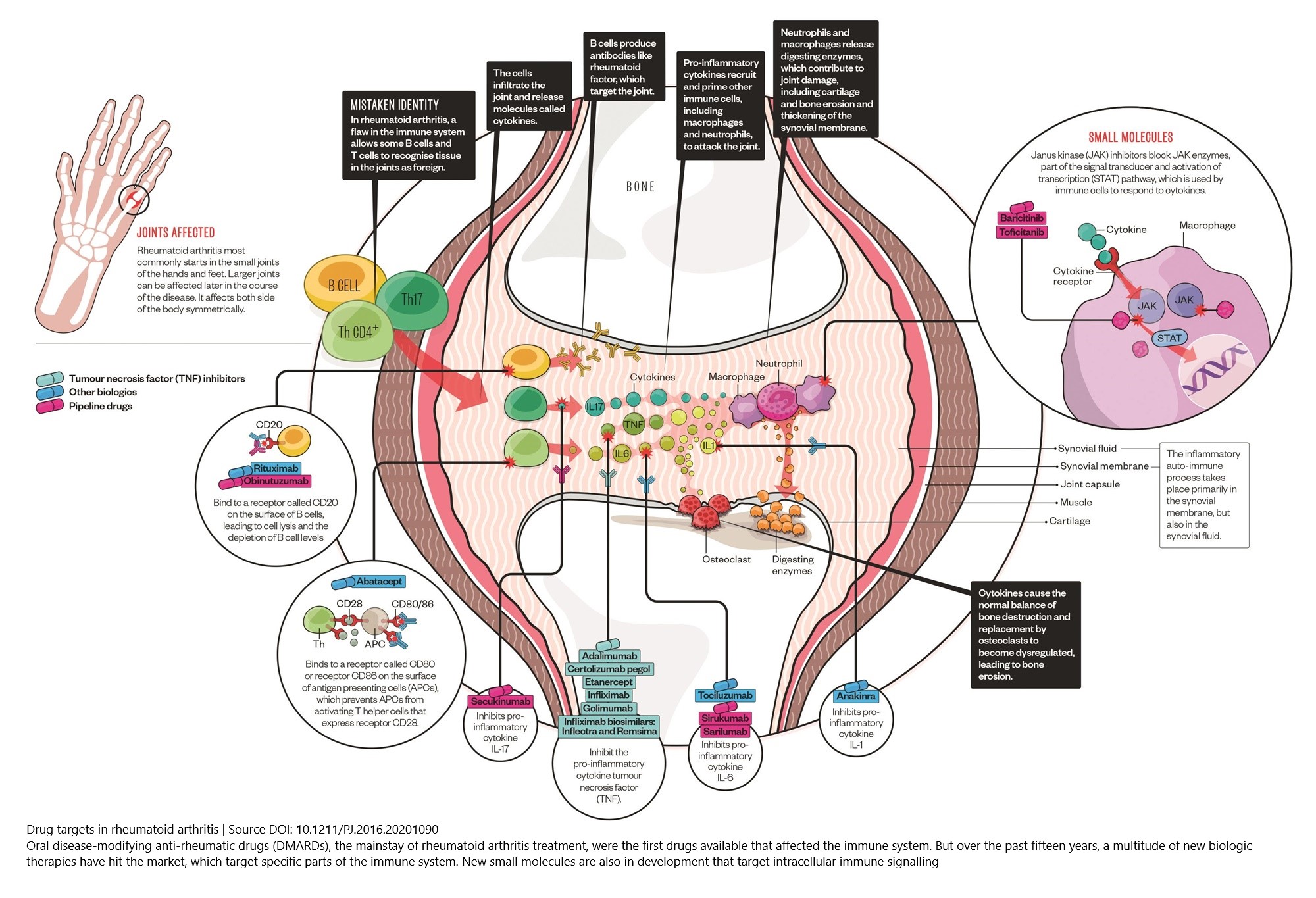
(Source DOI: 10.1211/PJ.2016.20201090)
In this online course, you can right mouse click on the image titles and choose “Open link in a new tab” in order to see a bigger version of the images and to zoom in.
2.1.1. A first look at T cell gene expression with the R2 platform
Data used:
- R2 dataset: Disease Rheumatoid arthritis subset (drugs) - Okuzono - 75 - deseq2 - gpl17303
- Description: 75 blood and synovial T cell samples of RA patients with rheumatoid arthritis
Techniques used:
- RNA Seq
References
Analysis used
- One Gene View
This green button will open up the Google form with which you can submit your answers for the first section. Only the questions with a R2D2 icon in front of them will have to be submitted.
Let’s take a first glance at the platform.
- Open a (preferably Chrome) browser and go to the webaddress: r2.amc.nl
- You don’t need to login for this course. You can click on the grey Use R2 without an account button just
underneath the sign in box.
However, when you do register to the platform and log in with your credentials, more datasets and analyses will become available to you. In order to register either use the blue Register a free account button on the login page or, if you are already on the main page, use the red link in the left side menu.
The four numbered boxes in the middle of the R2 main page allow you to choose a dataset and a type of analysis. In box 2 you can see that a dataset can be selected. We will be using a dataset of Okuzono that focuses on the disease Rheumatoid arthritis and that contains 75 samples.
- Click on the textfield of the currently selected dataset in box 2 and you will see a grid pop up.
This grid shows the datasets that are available to you. Every row is a dataset and every column contains a characteristic. In order to find datasets of interest, you can use the filter and sorting options next to and directly underneath the column headers.
- Type Okuzono in the textfield underneath the header Author and click the row of the dataset with 75 samples (column N).
- This dataset is now selected and you can read more background information about the dataset in the information panel underneath the grid.
- To use this dataset for analyses, click the blue button Confirm selection.
In box 3 you can select an analysis to perform on the selected dataset. Let’s have a first look.
- The default analysis is View a gene (box 3). Keep this setting and click Next in box 4.
- You now see the Adjustable settings box. Type in the textbox Search by gene of the setting Gene / Reporter: CD4.
- The pop-up dropdown shows all the available reporters of this dataset that contain the keyword CD4. Click on CD4 / 11829_2914 and you will see that the reporter textfield on the right is filled in automatically.
- Click the Submit button to obtain the result: a plot that shows you the gene CD4 expression values (log2, y-axis) for each sample (x-axis).
At the bottom of the page, you find the Adjustable settings box again. Many result pages allow you to adjust your analysis quickly from the same page. Here you can, for instance, change the gene that you want to look at, but also many other settings are available.
- Change the setting Transformation from Log2 to None and hit the Submit button in order for the adaptation to take effect. Now the plot shows you the untransformed expression values. You can see how the log2 scale on the y-axis might change your perspective of the same information: the log2 values in the lower range of the expression values are more spread out, it magnifies the relative differences between low expression values. For high expression values, the log2 transformation compresses the data.
Directly underneath the x-axis of the plot you can see colored blocks. These are different types of annotation. In R2
the samples of a dataset can be annotated with extra information, such as clinical data of patient samples, or biological characteristics of cell samples.
Each group of annotated data is called a track in R2. You will see the annotation often displayed underneath a
plot or by hovering over a plot. In this case, even more tracks are shown if you hover your mouse over the
dots in a plot.
- Try it out with your mouse: hover over the colored blocks of a sample underneath the plot, then also hover over the sample’s dot in the graph.
- Also, switch back to the log2 transformation. Don’t forget to Submit any time that you change a setting.
These tracks can be used in most of the analyses in R2 to add a layer of complexity. Tracks allow you for instance to filter datasets, to compare groups of samples, to color scatter plots of samples with meta information. Also, tracks enable you to correlate genomics patterns in your data, for instance to different phenotypes or demographic characteristics.
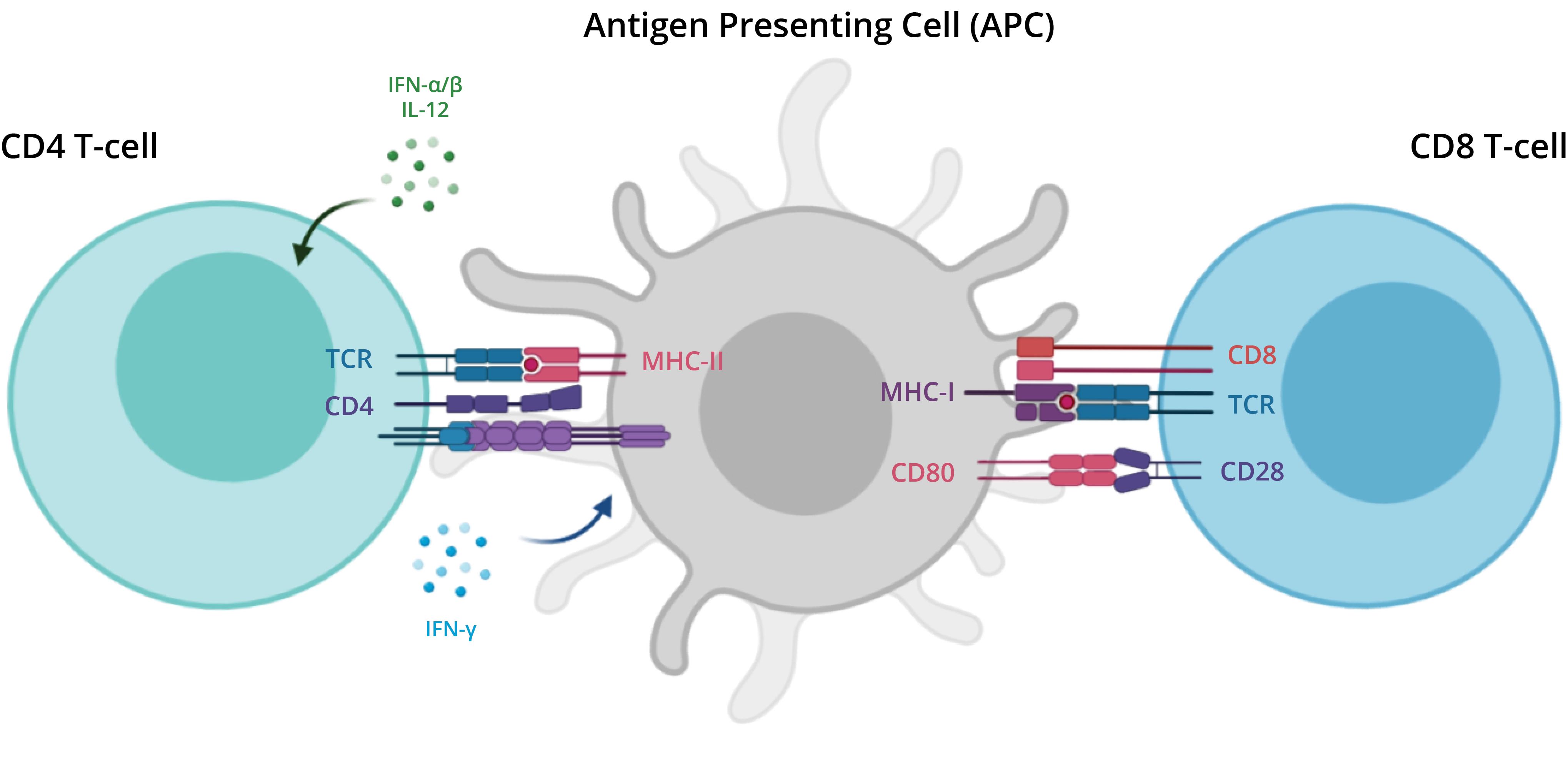
APC and T-cells

There are two major types of T cells: the helper T cell and the cytotoxic T cell. The helper T cells aid other cells
of the immune system by releasing regulating molecules, called cytokines.
With the help of protein complexes found on the surface of T cells, T cell receptors (TCRs), T cells recognize
specific antigens, which are molecules that are found on the surface of pathogens or abnormal cells.
An antigen presenting cell (APC) binds to the T cells and presents fragments, or peptides, of the antigen. The TCR
requires co-receptors in order to establish a stable connection to the APC. For instance, helper T cells express the
CD4 co-receptor and cytotoxic T cells express the CD8 co-receptor (gene name: CD8A). Although most T cells express
either CD4 or CD8, some express both and some do not express either.
![]() Look at the t-cell track underneath the graph. The two colors represent two different t-cell types. Hover with your mouse over the two different colors of this cell type annotation row. Which cell types are present in the dataset?
Look at the t-cell track underneath the graph. The two colors represent two different t-cell types. Hover with your mouse over the two different colors of this cell type annotation row. Which cell types are present in the dataset?
![]() Do you notice anything different about the expression levels of CD4 between the
two cell types?
Do you notice anything different about the expression levels of CD4 between the
two cell types?
![]() Now hover over the tissue track, which two tissue types can be found in this
study? Look back at the introduction of this course in which the hypothesis of Lee at al (2020) is provided, about the inflammatory responses in these tissue types.
Now hover over the tissue track, which two tissue types can be found in this
study? Look back at the introduction of this course in which the hypothesis of Lee at al (2020) is provided, about the inflammatory responses in these tissue types.
Tumor necrosis factor‐alpha (TNF‐α) is a proinflammatory cytokine that plays a pivotal role in regulating the inflammatory response in rheumatoid arthritis (RA).
To gain an initial understanding in how this cytokine relates to different tissue and cell types, we take a look at the expression values of gene TNF. We can take a shortcut route underneath the CD4 graph while we also change some other plot settings.
- Scroll down underneath the CD4 gene expression graph to find the Adjustable settings box.
- We can make use of the dataset’s annotations to view the results of our samples in groups. At the top of the Adjustable settings box change Analysis type from single gene to gene vs track and switch the Track setting to tissue (2cat) to separate the samples of the tissue blood from those of synovial fluid.
- Type TNF instead of CD4 in the Search by gene textbox of Gene / Reporter and select the first value TNF / 11829_18627 from the dropdown list of available genes / reporters.
- In order to have a look at the adjustments so far, click Submit for the adjustments to take effect.
- Scroll down again to change one more setting: in the Graphics settings adjust Graph type: to Box/dot plot (dots) and Color mode (groups): to Color by Track.
- Again click Submit for the adjustments to take effect.
The dots in the boxplot show the individual value of each sample, which is a good way to stay aware of the
distribution of the raw data points.
Often you use a boxplot to assess whether the expression values of a particular gene differ between groups of samples and to quickly identify their average values, outliers, the dispersion of the data set, and signs of skewness.
Next to the visual representation, R2 also provides this statistical information in textual format.
- Hover your mouse over each box to compare the summarizing values of the two groups.
The two groups clearly show different trends in their expression values of TNF. But how do we know whether the group
means vary significantly, i.e. by more than random chance allows? To answer that question R2 shows you the results
of an analysis of variance (ANOVA): you can find the F-value, the test statistic of the ANOVA test, and the p-value
of the ANOVA test in the table underneath the plot.
![]() What can you conclude about the expression of the gene TNF in blood tissue versus synovial fluid?
What can you conclude about the expression of the gene TNF in blood tissue versus synovial fluid?
Remember that one of the main questions of this study was whether peripheral blood samples can replace samples of
synovial fluid that are hard to obtain from patients. Of course, we can’t say anything about that yet, but we gained
some awareness of the tissue specific expression levels.
APC and T-cells
T cells originate from hematopoietic stem cells in the bone marrow that migrate to the thymus. They undergo several developmental stages to differentiate into mature, naïve T cells. These exit the thymus and enter the peripheral circulation, where they undergo further maturation and differentiation into effector or memory T cells upon encountering antigens presented by antigen-presenting cells.

Figure 3: Differentiation of T-cells, each subtype having its specific role in the immune system.
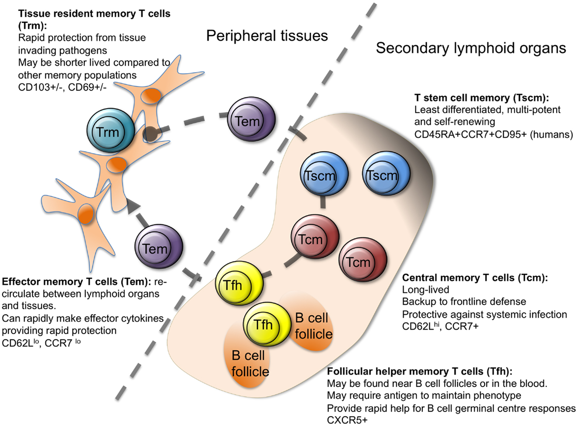
By developmental stage, CD4+ T cells are classified into four stages: naïve (Tn), stem cell memory (Tscm), central memory (Tcm) and effector memory (Tem), whereas CD8+ T cells are classified into five stages: Tn, Tscm, Tcm, Tem and CD45RA-positive effector memory (Temra).
This heterogeneity among T cells makes it challenging to identify the specific cell subsets and states that drive RA pathogenesis.
- Under your latest graph, change the setting Track to t-cell-stage-type.
- Click Submit.
![]() Which T-cell subtype has the lowest expression?
Which T-cell subtype has the lowest expression?
![]() Which T-cell subtype has the highest expression of TNF?
Which T-cell subtype has the highest expression of TNF?
Naive T cells are in a quiescent state and have not undergone differentiation into effector or memory T cells. Effector T cells, including effector memory T cells, are specialized to carry out immune responses, including cytokine production such as TNF.
- Submit your Google form with answers of the above section
2.1.2. Exploring relevant annotation of a dataset
Analysis used
- Cohort Overview
This button will open up a Google form for section 1.2.2.
We have seen before that the samples of a dataset can be annotated with extra annotation, or tracks.
To get a better overview of the available annotation of a dataset, we can use the tool Cohort Overview in R2.
- Go back to the main page (in the upper left corner of the page, click on Go to: Main) and select Cohort Overview as type of analysis in box 3. Click Next.
R2 presents the Okuzono dataset samples with its available annotation in a table at the bottom of the page. Each pie chart above the table shows a different available track.
- Hover your mouse over the different slices of the tissue annotation pie chart. What percentage of the samples is synovial fluid and what percentage is blood tissue?
- Explore the other pie charts as well: hover with your mouse over the slices and click on a slice to select that group of the samples. Above the main pie chart you can read the number of samples in your current selection (the “n= “ number). Also, you will see which selection you have made in the box Applied filters. Note how the table at the bottom adapts the overview based on your selection. You can click on the button Clear Filters to undo your selection.
![]() How many (n=..) synovial fluid samples are present in this dataset?
How many (n=..) synovial fluid samples are present in this dataset?
![]() And how many samples are CD4 Effector Memory T cells (Tem) in the blood tissue? (Hint: you will have to apply 3 different filters)
And how many samples are CD4 Effector Memory T cells (Tem) in the blood tissue? (Hint: you will have to apply 3 different filters)
- Please, submit your form. Thanks!
2.2. Effects of treatment
Now that we have a better understanding of the biology involved in rheumatoid arthritis, let’s have a look if we can find any effect of rheumatoid arthritis treatments.
Data used:
- R2 dataset: Disease Rheumatoid arthritis (drugs) - Lauwerys - 40 - MAS5.0 - u133p2
- Description: Paired synovial biopsy samples were obtained from the affected knee of early RA patients before and 12 weeks after initiation of Tocilizumab (n=12) or Methotrexate (n=8) therapy
References
Analyses used
- Cohort Overview
- One Gene View
2.2.1. Explore the provided information
This button will open up a Google form for section 1.3:
How does treatment effect gene expression? Let’s have a look at a dataset of Lauwerys et al. In the dataset we can find samples taken from the synovial fluid in the knee of 20 early RA patients, both before and after treatment.
- Go to the Main page of R2 and click on the text area in box 2 that currently contains the Okuzono dataset title.
- The popup window appears that shows all the available datasets in the grid again. Type in the text field under Author the name of the author of the data set: Lauwerys
- Click on the row of the dataset of our interest with 40 samples. Underneath the grid you can see more details about the study (you don’t have to read it yet). Note that in this information overview you can also find a Pubmed link to the study.
- Click on the blue Confirm Selection button in the grid.
First, we take a look at the provided annotation. Let’s start with the dataset Cohort Overview.
- In box 3, select the Cohort Overview, click Next and explore the available annotation.
Since this dataset is treatment related, let’s plot the data to see if treatment has any effect according to this study.
- Go back to the main page (click Main in the upper left corner). Choose the analysis Correlate Gene with track, click Next.
Throughout R2 you can view the extra information of the selected dataset, with a click on the i information balloon behind the dataset title on the top of the page.
- Click on the information balloon i and take a note of the cytokines & chemokines that are mentioned in the description box. Close the box with the x in the upper right corner.
- Fill in IL6 in the Search by Gene field of the Gene / Reporter setting, i.e. one of the genes that were mentioned to be down regulated by treatment. The “-” can be left out of the gene name in R2, e.g. “IL-6” becomes “IL6”. Choose the appropriate gene from the dropdown list.
- Choose Track: therapy (2cat) and change Graph type to XY plot. This way we can find out if there is a correlation between the values before treatment and after treatment. Also, R2 will plot the data points in an XY plot with the gene expression value on the Y axis and the treatment groups on the X axis.
- Let’s color the data by the drug treatment: Color mode Color by Track and Color track drug (3 cat), then click Submit.
Every patient had a sample taken before the start and after 12 weeks of therapy; it is a paired test. For each patient there is one dot for the IL6 gene expression before treatment (colored blue, annotated with therapy: no, duration: t0, drug: untreated) and one dot for the IL6 gene expression after treatment (colored green or red, annotated with therapy: yes, duration: t12, drug: tocilizumab or methotrexate). The track identifier tells you to which patient the sample belongs.
- Hover your mouse over a couple of data points in the graph to see that the tracks therapy and duration are lined up with the according values. Also take note of the track identifier.
To see the effect of treatment on each patient, it would be more insightful to see the relation between data points that belong to the same patient. Also, we would like to see the statistical significance of treatment of the two different treatments.
- With Sample Paths we can connect the two samples of each patient with the format Samplename1,Samplename2; etc. Because it is rather labour intensive to get the correct syntax, we did this for you. Select all text from the text field below and copy-paste it in the field Sample Paths.
- To see the result click on Submit and take note of the results of the ANOVA test underneath the plot.
Let’s compare the statistics of the individual treatments. We make use of the Sample Filter and the track experiment, that tells you to which drug experiment each sample (including the untreated samples) belongs.
- Under the graph select for the setting Subset track the value experiment and in the pop up, check mtx (16), click ok. Click Submit
- Take note of the ANOVA results underneath the graph.
- Now change the Subset track to the other experiment. Click the red cross to deselect the previous value, from the dropdown select experiment and in the popup check the square tcz (24). Click ok and then in the settings box, click Submit.
- Take note of the results of the ANOVA test underneath the plot.
![]() What can you tell about the effect of the different treatments on the expression of this gene? Does this confirm or oppose the description of the study?
What can you tell about the effect of the different treatments on the expression of this gene? Does this confirm or oppose the description of the study?
Optional:
- Change the gene to a different gene that you can find in the description of the study, or that you yourself wonder about. Don’t forget to submit the settings in order to see the changes.
![]() Which gene did you choose and what can you tell about the effect of treatment on the expression of this gene?
Which gene did you choose and what can you tell about the effect of treatment on the expression of this gene?
2.2.2. Exploring differentially expressed processes
We now want to know which pathways are affected by treatment with tocilizumab.
- From the main page, select the analysis Differential Expression between two groups, click Next
- Choose Group by: therapy (2 cat).
- For Subset track choose experiment and check tcz (24). Click ok and click Submit. Extra settings will pop-up.
- Choose Group 1 no (12) and Group 2 yes (12).
- Because we won’t have many samples, we will not correct for multiple testing. Under Statistics change Corr. multiple testing: to No correction. Click Submit.
The list shows the genes that are differentially expressed between the patients before treatment and after treatment. Above the table you can see how many genes have been found to be significantly differentially expressed with a p-value of at most 0.01.
- On the right side of the table, buttons allow to perform further analyses on the obtained list of differentially expressed genes. To see in which processes these genes are involved, we click on Gene Ontology Analysis button.
The analysis connects to the Gene Ontology knowledgebase (http://geneontology.org/), “the world’s largest source of information on the functions of genes”. The knowledgebase contains information about which genes are involved in which biological processes.
The R2 Gene Ontology algorithm checks for which processes the involved genes are overrepresented in our list of
differentially expressed genes, i.e. it looks at the probability that the number of up or down regulated genes of
that process, occur in our list by chance (randomly).
In this table each row contains information of one biological process: its name, the p-value of the overrepresentation and the involved genes that are up (yes >= no) or down (yes < no) regulated with therapy. Above the table you can find the meaning of the red and green color coding.
![]() What kind of processes seem to be affected by treatment?
What kind of processes seem to be affected by treatment?
![]() Are the genes that are involved in these processes mostly higher or lower expressed after treatment? (Hint: Look at the color scheme above the table)
Are the genes that are involved in these processes mostly higher or lower expressed after treatment? (Hint: Look at the color scheme above the table)
The page with the list of differentiating genes is still open in a tab. On this page many buttons and links allow you to visualize and analyze the result further. Try these options, or try to interpret the results that you obtain with one of the buttons on the right:
- From the list of differentiating genes, choose one of the top genes and hover your mouse over the glass icon in front of the gene to read information about the gene. Now click on the icon to be taken to the One Gene View for this gene. Of course you can adapt the graph again with the menu underneath the graph.
- On the page with the list of differentiating genes, still open in the other tab, click on the button Plot all genes (xy, vulcano etc.)
- Underneath the plot, change Plot type to Vulcano plot.
- Hover with your mouse over some dots furthest to the upperleft corner in the plot to read their names. Compare those names with the list of differentiating genes.
- In the Adjustable settings box, write the name of a gene in the text box of Mark genes and hit Enter to see if you can locate the gene in the vulcano plot. (E.g. you can use one of the genes from the dataset description “We found that Tocilizumab induces a significant down-regulation of genes included in specific pathways: cytokines & chemokines (e.g. IL-6, IL-7, IL-22, CCL8, CCL11, CCL13, CCL19, CCL20)”)
- To see what the expression difference looks like of a gene, click on any dot in the Vulcano plot, first with a left mouse click to mark the gene in the plot in an interactive way. Then right click to see the expression of the gene in the two different therapy groups “no” vs “yes”.
- Back in the tab with the vulcano plot, in the Adjustable settings box, click on Search GO button. In the GO description column you can type in the white textfield (directly underneath the header) to search for particular keywords and to find a Gene Ontology set of interest. Let us try the keyword immune. The table adjusts to those GO sets that contain the keyword immune. Select any GO set (e.g. activation of immune response) with the Select button in front of that row and click the button Update Genes to see if the genes marked by this GO set are mainly up- or downreguated.
- On the tab with the list of differentiating genes, now click the button Heatmap (zscore) to get an overview of all the genes and the (unsupervised) group separations in a Heatmap.
- Redo the Differential Expression between groups analysis and Gene Ontology analysis for the other treatment. Thus choose for Subset track experiment and check mtx (16), while keeping all the other settings the same. Don’t forget to switch off the Corr. multiple testing.
![]() What results do you get with this treatment? Read the dataset description again. Do your results correspond with results of the study?
What results do you get with this treatment? Read the dataset description again. Do your results correspond with results of the study?
- Please, submit your form. Thanks!
2.3. Final remarks / future directions
You have reached the end of this course. Feel free to try one of the (Graduate) Student Courses that you can find in the sidebar of this page https://r2-training-courses.readthedocs.io/en/latest/.
We hope that this course has been helpful. If you want to have your genomics data visualized and analyzed using the R2 platform you can always consult r2-support@amc.nl
The R2 support team.